
My Thoughts
•
The most interesting contribution is to interpret their model as a general representation of previous architectures for point-cloud tasks.
•
Also it was interesting to view their design of EdgeConv as balance the effect of local and global information of vertices.
•
Drawing graphs & K-NN for every layer might be exhaustive. Yet, these are (or can be) easily done on CUDA based on some Torch functions. But how could they achieve way faster time that PointNet++ and PCNN?
•
While their dynamicity can bring rich context for various tasks, it might harm the convergence of the training on the first step. There could have been extensive experiments to get the optimal training environment.
Applicability to PBR
•
The graph's dynamicity can be extended by using path graphs for temporal rendering. The model can still handle new vertices and edges from the next sample or the next frame.
•
Their final model (Eq.(8)) resembles the model of post-processing for MC denoising. The difference is that the inputs (features) are optimized for this work while post-processing (pixel radiances) doesn’t. Still, such method could have contributed to a more optimal result by reducing any bias.
Problems to Solve
•
Recent PointNet-based methods treat points independently → Fail to capture local features
◦
Even though variations include locality (i.e. using neighbor points for embedding)
•
Grid-like representations to overcome the irregular distribution of point clouds requires lots of memory and leads to artifacts (aliasing).
Constructing Graph
1.
Construct a graph with points as vertices .
2.
Draw edges based on the K-nearest neighbor based on the distance .
Edge Convolution
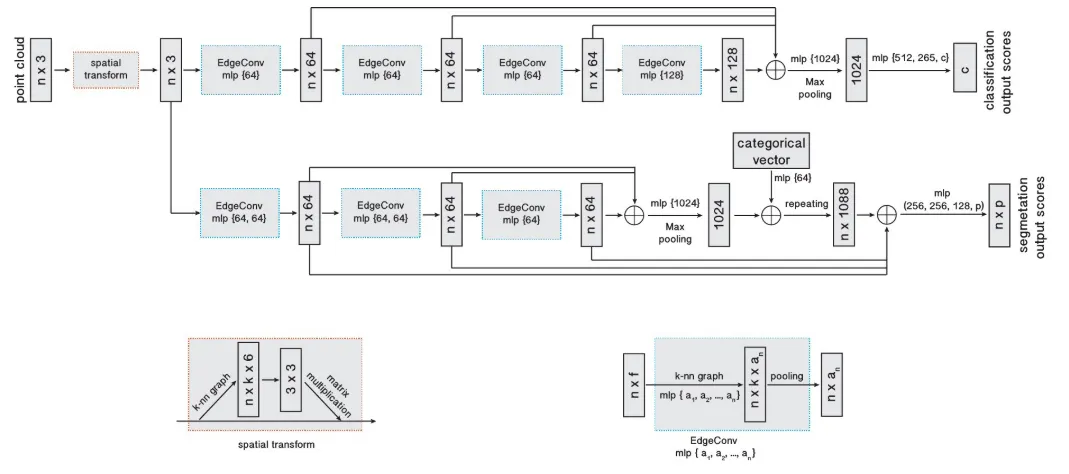
Overall architecture of DGCNN for classification & segmentation
1.
Calculate the edge features as , where is a trainable function
The asymmetric structure resembles balancing the local information and the global information during training.
This is implemented as MLP and applied to vertices via shared MLP.
2.
Update the vertices as .
3.
Update edge features
4.
And so on…
