My Thoughts
•
Using graphs is an interesting approach. Recent works and classic works approach paths as a sequence or a single concatenated feature but not as graphs(actually trees). Furthermore, using a graphs-like structure for reducing noise can be popular.
•
However, there are main concerns. Firstly, constructing a graph for a high-res image can be cumbersome. Secondly, reducing bias for 3D GNN can be hard (this work doesn’t have a bias). It can be easily handled by dividing the image. The second concern can be the novelty of future work.
•
Reducing bias via final gather is an important method. This rises the point where post-denoising works make. We can investigate more to a more unbiased method.
•
This work has a limitation of clamping the value based on MIS and complex BSDF. When applying GNN on path graphs, we might need to think of cases where complex scenes can make the training hard to converge.
Motivation
•
Recent reconstruction methods (path guiding, denoising) are based on final radiances. We can use more information in path-space which will be useful for sparse samples.
•
Recent sample reusing works are done locally. This work aims to provide a global path reuse concept based on K-NN vertices linked with neighbor edges.
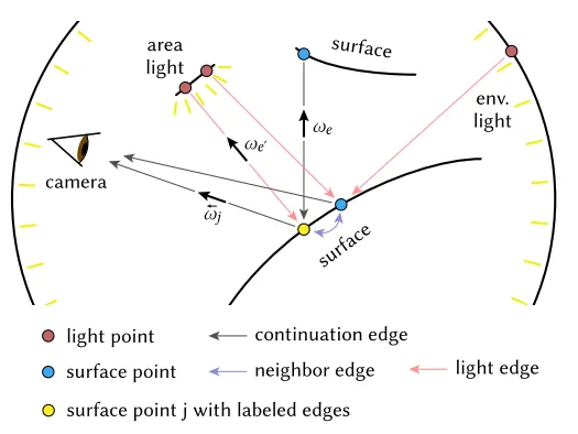
Construct Path Graph
•
Light edge (LE) = Edge with endpoint of light source
•
Continuation edge (CE) = Edge with endpoint of surface
•
Neighbor edge (NE) = Edge linking K-nearest vertices
•
Further notation combines NE and LE/CE as below.
: Set of vertices linked with shading vertex via neighbor edges
: Light/Continuation edges with endpoints in
Aggregation & Propagation
•
Separate direct/indirect radiances and individually aggregate them. (Similar to Radiosity)
•
Get weight for each sampled result based on balance heuristics
•
Aggregation is done based on Multiple Importance Sampling → Unbiased approach
Direct radiance: where
Indirect radiance: where
Note that for indirect radiance, each sample is from independent sampling techniques. Thus we sum them up directly (without weighting).
•
Update outgoing radiance of for all
These process takes . But the authors reduce to by caching the pdf calculations. To do so, the steps are reduced as below
•
Get marginal density of sampling for all continuation edges
•
Calculate direct and indirect radiances based on aggregation above.
Iterative Approach based on Linearity
•
Aggregation step can be viewed as simple linear system .
•
Authors apply Jacobi method to iteratively update (radiance in this case) base do the linear system
◦
To guarantee convergence, they clamp the eigenvalues of to 1.
•
Iteration is done until converge.
Final Gather
•
To remove correlation of nearby points, the final iteration is done with .
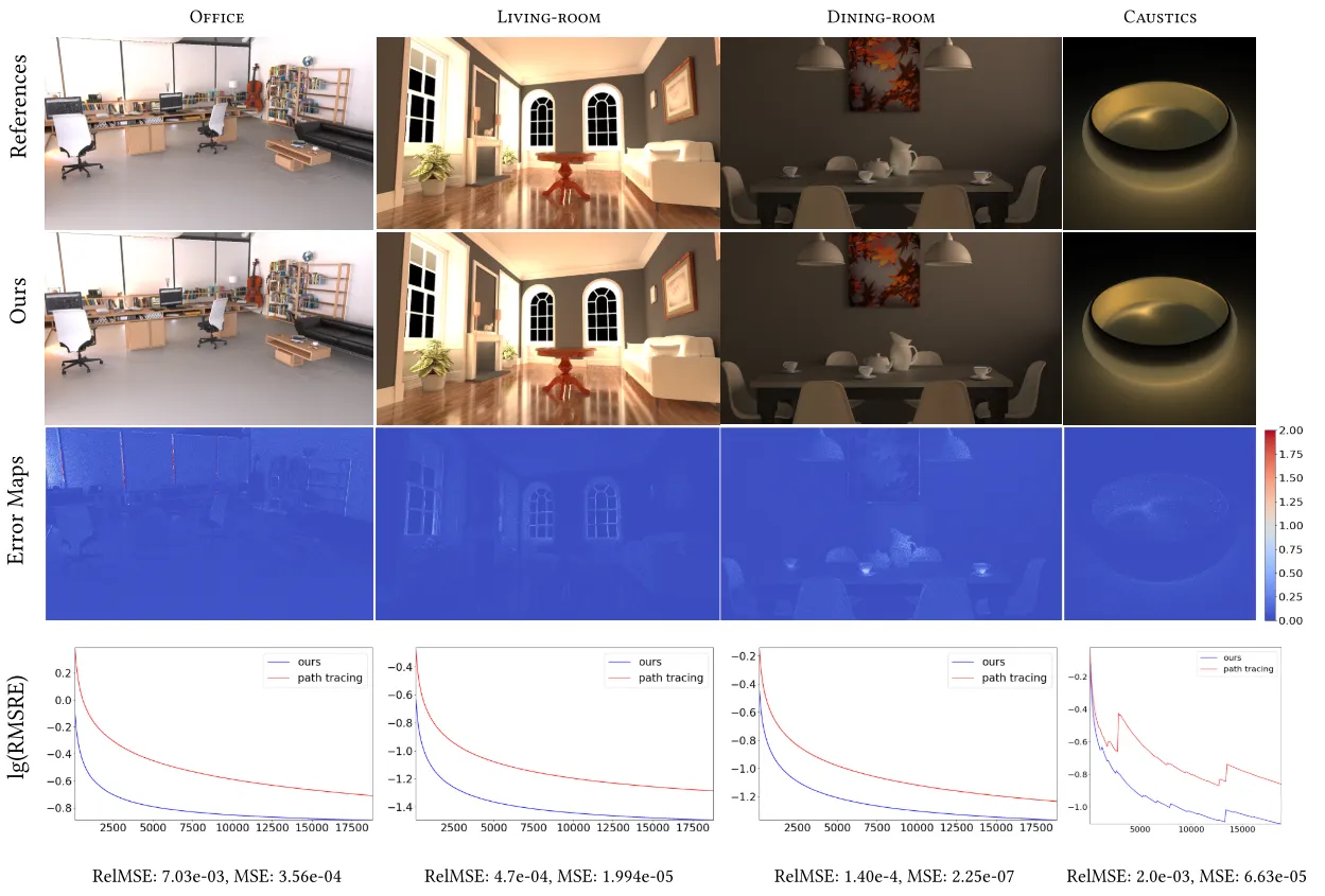
Results
•
Even though bias (should) exist, the method converges well.