Continuous Multiple Importance Sampling[ToG20]

Theme

논문

Type

테마글

Status

Post

분야

Monte Carlo Noise Reduction

중요도

⭐

2 more properties

My Thoughts

•

It was hard to think of the demand for continuous technique space in rendering, but this paper has shown its various applications. Great work.

•

However, to achieve unbiasedness there still requires some computation, especially PDF computation. For expensive BSDF this might take a long time.

•

Also, the paper compares the path-space filtering with quite out-of-time work. This makes the result and the performance less outstanding. However it’s understandable since there are not much path-reuse works directly working on samples and paths.

Review (Discrete) Multiple Importance Sampling (DMIS)

Given the following rendering equation (only scattering) and an Estimator.

L_o(x',w'_o )=\int_{\mathbf{S}^2}{f_s(\mathbf{x}', \omega;_i\rightarrow \omega'_o)L_{e,i}(\mathbf{x}', \omega'_i)d\omega_i}

Usually starting with two sampling strategies

•

BSDF Sampling

probability density set proportional to BSDF

f_s

, or any other BSDF approximation

good for highly polished BSDF

bad for extreme light sources (small, multiple light sources)

•

Direct light sampling

among visible light sources, choose the point

V(\mathbf{x}\leftrightarrow\mathbf{x}')\frac{|\cos(\theta_o)\cos(\theta'_i)|}{\lVert{\mathbf{x}-\mathbf{x}}\rVert^2}

good for dealing with various light sources

bad for complex BSDF

Among these, there can be various ways to choose the sampling domain and sampling density for a certain integrand.

How can we combine the samples from these various sampling properties with the least variance?

Given an integral and an estimator:

I=\int_\chi{f(x)dx},~~~~~~\langle I \rangle_n=\frac{1}{n}\sum^n_{i=1}\frac{f(x_i)}{p(x_i)}

Multi-sample estimator is as below:

F=\sum^n_{i=1}\frac{1}{n_i}\sum^{n_i}_{j=1}w_i(X_{i,j})\frac{f(X_{i,j})}{p_i(X_{i,j})}

The weight function

w_i(X_{i,j})

balances the contribution of each sample of sampling density

f(X_{i,j})/{p_i(X_{i,j})}

. For unbiasedness, the weight function should follow the properties

(1)~~~~~~~~\sum^n_{i=1}w_i(x)=1 ~~ \text{whenever} ~ f(x)\neq 0 \\ (2)~~~~~~~~w_i(x)=0~\text{whenever}~p_i(x)=0

It is known that the following balancing heuristics gives the least variance for multiple-sample estimator

\hat{w}_i(x)=\frac{n_ip_i(x)}{\sum_k n_kp_k(x)}

Continuous Multiple Importance Sampling (CMIS)

Conventional DMIS deals with fixed number of sampling strategies. The paper extends the sampling strategies into a continuous space, where sampling strategies are in the continuous technique space

\mathcal{T}

Then the integral and the estimator can be written as below

I=\int_\mathcal{X}\int_\mathcal{T} {w(t,x)dtf(x)dx}=\int_\mathcal{T}\int_\mathcal{X} {w(t,x)f(x)dxdt},~~~\langle I\rangle_{CMIS}=\frac{w(t,x)f(x)}{p(t,x)}=\frac{w(t,x)f(x)}{p(t)p(x|t)}

p(t)

is the probability of sampling a technique

t

p(x)

is the probability of sampling point x, and

p(t,x)

is a joint PDF.

Similary to DMIS, weight function of CMIS also shares the similar condition

(C_1)~~~\int_\mathcal{T}w(t,x)dt=1~~\text{whenever}~~f(x)\neq 0 \\ (C_2)~~~w(t,x)=0~~\text{whenever}~~p(t,x)=0

Also similary to DMIS, CMIS shows less variance when using balance heuristics instead of uniform weight.

\hat{w}(t,x)=\frac{p(t)p(x|t)}{\int_\mathcal{T}p(t')p(x|t')dt'} = \frac{p(t,x)}{\int_\mathcal{T}p(t', x)dt'}=\frac{p(t,x)}{p(x)}

By doing so, CMIS can deal withan uncountable set of sampling techniques, while DMIS can deal witha countable infinite set of techniques by

n\rightarrow\infty

Stochastic Multiple Importance Sampling (SMIS)

However, calculating the weight function requires the computation of the marginal PDF of

p(x)

in the denominator. As always, integration on arbitrary PDF is most unlikely to be done in closed form.

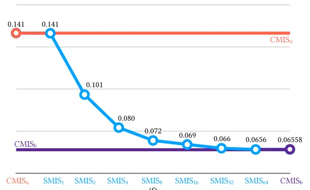
Therefore, this paper approximates it as an average of existing samples

(t_i, x_i)

, similar to sample-reuse techniques of

t_i\sim p(t_i)

\frac{1}{n}\sum^n_{i=1}\frac{p(t_i,x_i)}{\int_\mathcal{T}p(t,x_i)dt}\approx\frac{1}{n}\sum^n_{i=1}\frac{p(t_i,x_i)}{\frac{1}{n}\sum^n_{j=1}\frac{p(t_j,x_i)}{p(t_j)}}\cdot\frac{f(x_i)}{p(t_i, x_i)}

LHS refers to n-sample CMIS, and RHS refers to the approximation with SMIS.

And the estimator becomes

\langle I\rangle_{SMIS}=\sum^n_{i=1}\frac{\dot{w}(t_i,x_i)f(x_i)}{p(x_i|t_i)}=\sum^n_{i=1}\frac{f(x_i)}{\sum^n_{j=1}p(x_i|t_j)}

The new estimator is biased to approximate the estimator of CMIS, but eventually unbiased to approximate the original integral. Given n samples, SMIS requires

n^2

PDF computation in the denominator. This requires much overhead. Therefore, one should find a balance for total

N

samples, how much samples we require for approximation (

n)

and how much realization do we use (

N/n)

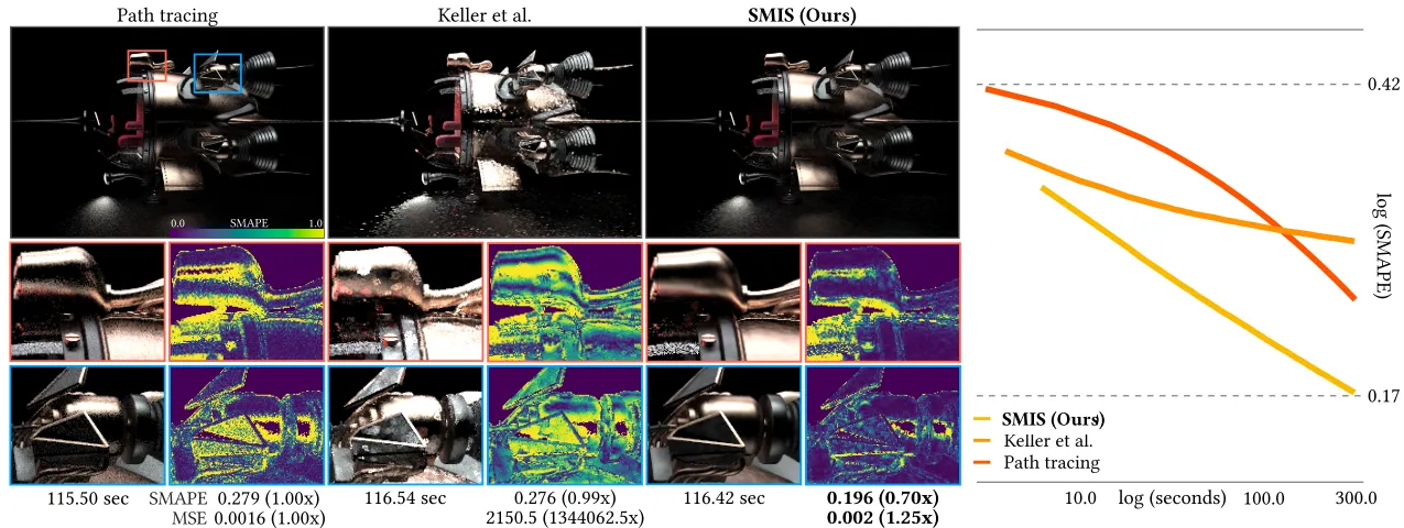
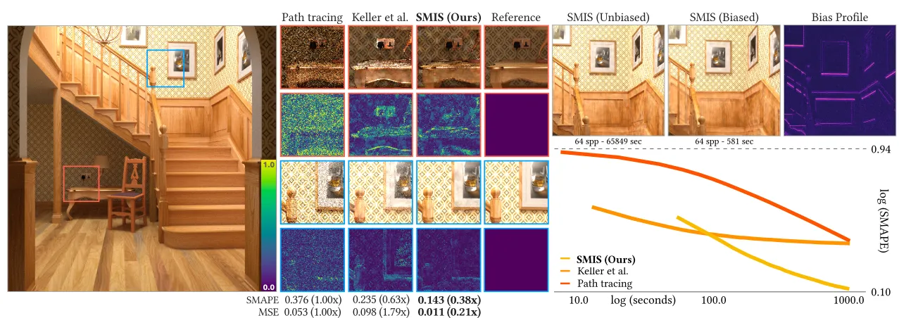
Path-space filtering (Path Reuse)

Formulation of CMIS and SMIS can be used for path-space filtering. Unlike previous methods, this method gives both better convergence and unbiasedness.

We can formulate the rendering a pixel

I

with light transport of uncountable infinite path space

\mathcal{P}

by decomposing a path

\bar{p}

into two subpaths (prefix, suffix) =

(\bar{y},\bar{z})

as below.

I=\int_\mathcal{P}f(\bar{x})d\bar{x}=\int_\mathcal{P}f_e(\bar{y})\int_\mathcal{P}f_l(\bar{y},\bar{z})d\bar{z}d\bar{y}=\int_\mathcal{P}f_e(\bar{y})I(\bar{y})d\bar{y}

Supposing we have paths

\bar{y_i}\bar{z_i}

, we want to reuse suffices to link a given prefix

\bar{y}

Previous works formulate the estimator as below.

\langle I\rangle=\frac{f_e(\bar{y})}{p(\bar{y})}\langle I(\bar{y})\rangle_n = \frac{f_e(\bar{y})}{p(\bar{y})}\sum^n_{i=1}w(\bar{y},\bar{z}_i)\frac{f_l(\bar{y},\bar{z_i})}{p(\bar{z}_i)}

And approximate the weighting function.

We can formulate this problem into CMIS.

I(\bar{y})=\int_\mathcal{P}\int_\mathcal{T}w(\bar{y}',\bar{z})d\bar{y}'f_l(\bar{y},\bar{z})d\bar{z}=\int_\mathcal{T}\int_\mathcal{P}w(\bar{y}',\bar{z})f_l(\bar{y},\bar{z})d\bar{z}d\bar{y}' \\ \langle I(\bar{y}) \rangle_{\tt CMIS}=\frac{1}{n}\sum^n_{i=1}\frac{w(\bar{y}_i, \bar{z})f_l(\bar{y},\bar{z}_i)}{p(\bar{y}_i)p(\bar{z}_i|\bar{y}_i)}

And the CMIS estimator can be approximated as SMIS estimator below.

\langle I(\bar{y}) \rangle_{\text{SMIS}}=\sum^n_{i=1}\frac{\dot{w}(\bar{y}_i,\bar{z}_i)f_l(\bar{y},\bar{z}_i)}{p(\bar{z}_i|\bar{y}_i)}=\sum^n_{i=1}\frac{f_l(\bar{y},\bar{z}_i)}{\sum^n_{j=1}p(\bar{z}_i|\bar{y}_j)}

Unlike previous work [Keller et al. 2014], this work weighs paths(samples) based on sampling densities (balance heuristics). Previous work weighs samples based on similarity in surface (position).